Regression based models

Motivating example

To motivate the general idea of regression based models, let us look at the data points in the picture below. The question is which assignment of a normalized risk score to these data points makes sense:

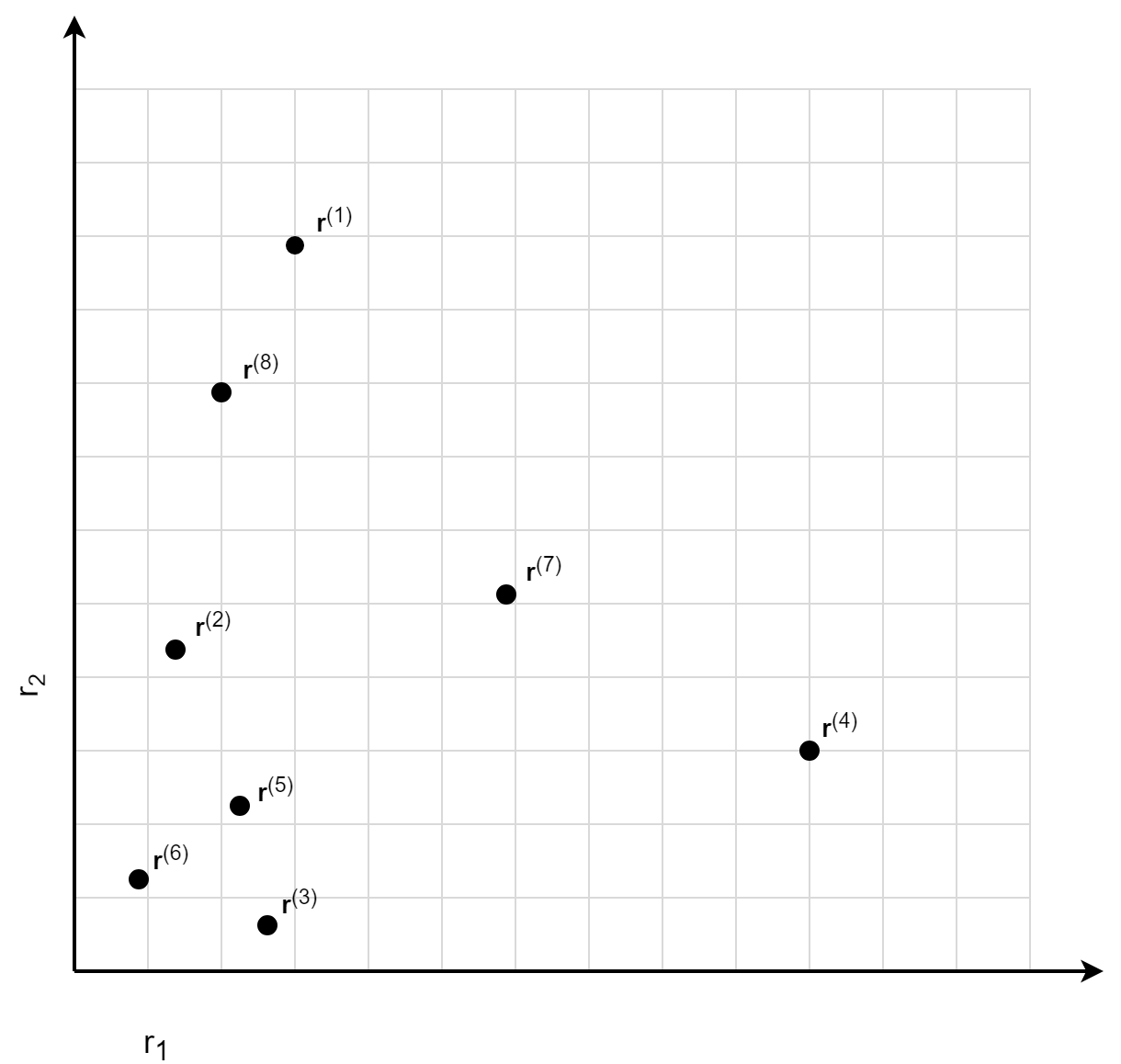
One possible answer would be:

• The data points r⁽¹⁾, r⁽⁷⁾ and r⁽⁴⁾ have the highest normalized risk score because they are the most extreme ones. No other data points are 'greater'.
• The data point r⁽⁸⁾ has the second highest normalized risk score, since only the data point r⁽¹⁾ is 'greater'.
• The data points r⁽²⁾, r⁽⁵⁾ and r⁽³⁾ are somehow similar, they all have the third highest normalized risk score.
• The data point r⁽³⁾ has the lowest normalized risk score.

The answer above is based on counting the number of data points that are 'greater than' the data point under consideration. The used 'greater than' relationship says that the data point r' is 'greater than' r if all plug-in risk scores r_i' of r' are greater than the plug-in risk scores r_i of r. For generalizing the argumentation above, we introduce the following notation:

• <_gt denotes the 'greater than' order relationship: r <_gt r' <=> r_i < r_i' for all i = 1, 2, ..., n.
• D denotes the set of all observed data points: D = {r⁽¹⁾, ... , r^(N)} with N as number of observations.
• D_gt⁽ⁱ⁾ denotes the set of all data points 'greater-than' the data point r⁽ⁱ⁾ : D_gt⁽ⁱ⁾ = { r ∈ D | r⁽ⁱ⁾ <_gt r}
• The size of a set S will be denoted by |S|

We then define: r_normalized( r⁽ⁱ⁾) = 1 - |D_gt⁽ⁱ⁾| / ( |D| - 1 ) .

Applying the formula for the normalized risk score to the data points, we receive:

r	Dgt	|Dgt|	rnormalized
r(1)	Dgt(1) = {}	0	1 - 0 / (8 - 1) = 1
r(7)	Dgt(7) = {}	0	1 - 0 / (8 - 1) = 1
r(4)	Dgt(4) = {}	0	1 - 0 / (8 - 1) = 1
r(8)	Dgt(8) = {r(1)}	1	1 - 1 / (8 - 1) = 0.86
r(2)	Dgt(2) = {r(1), r(8), r(7)}	3	1 - 3 / (8 - 1) = 0.57
r(5)	Dgt(5) = {r(1), r(7), r(4)}	3	1 - 3 / (8 - 1) = 0.57
r(3)	Dgt(3) = {r(1), r(7), r(4)}	3	1 - 3 / (8 - 1) = 0.57
r(6)	Dgt(6) = {r(1), r(8), r(7), r(4), r(2), r(5)}	6	1 - 6 / (8 - 1) = 0.14

Artificial response variable

The normalization problem itself is an unsupervised problem, since we do not have any response variable. We now use the counting approach described above to generate an artificial response variable y for every observed data point r⁽ⁱ⁾: y⁽ⁱ⁾ = 1 - |D_gt⁽ⁱ⁾| / ( |D| - 1 ) . By introducing the artificial response variable y⁽ⁱ⁾, we have turned the unsupervised problem into a supervised regression problem:

• We have a training data set {(r⁽¹⁾,y⁽¹⁾ ), (r⁽²⁾,y⁽²⁾ ), ..., (r^(N),y^(N) )} and want to learn a function N, y = N(r).
• The normalized risk score is the prediction of that function: r_normalized = N(r).

The big advantage is that there are many well-established techniques for solving a regression problem. Another important aspect is that the training data set {(r⁽¹⁾,y⁽¹⁾ ), (r⁽²⁾,y⁽²⁾ ), ... , (r^(N),y^(N) )} is fulfilling the Proximity property, so we expect that the prediction function N also tries to fulfill that property. In the following we describe two different normalization models that are based on solving the regression problem formulated above.

Ordinary least square normalization model

In the ordinary least square normalization model (OLS-model), we use a linear regression function N: r_normalized = N(r) = w^T· r + a, with a D-dimensional weight vector w and scalar intercept a. Furthermore, we use a squared loss function. The model parameters w and a will be computed by the gradient descent method.

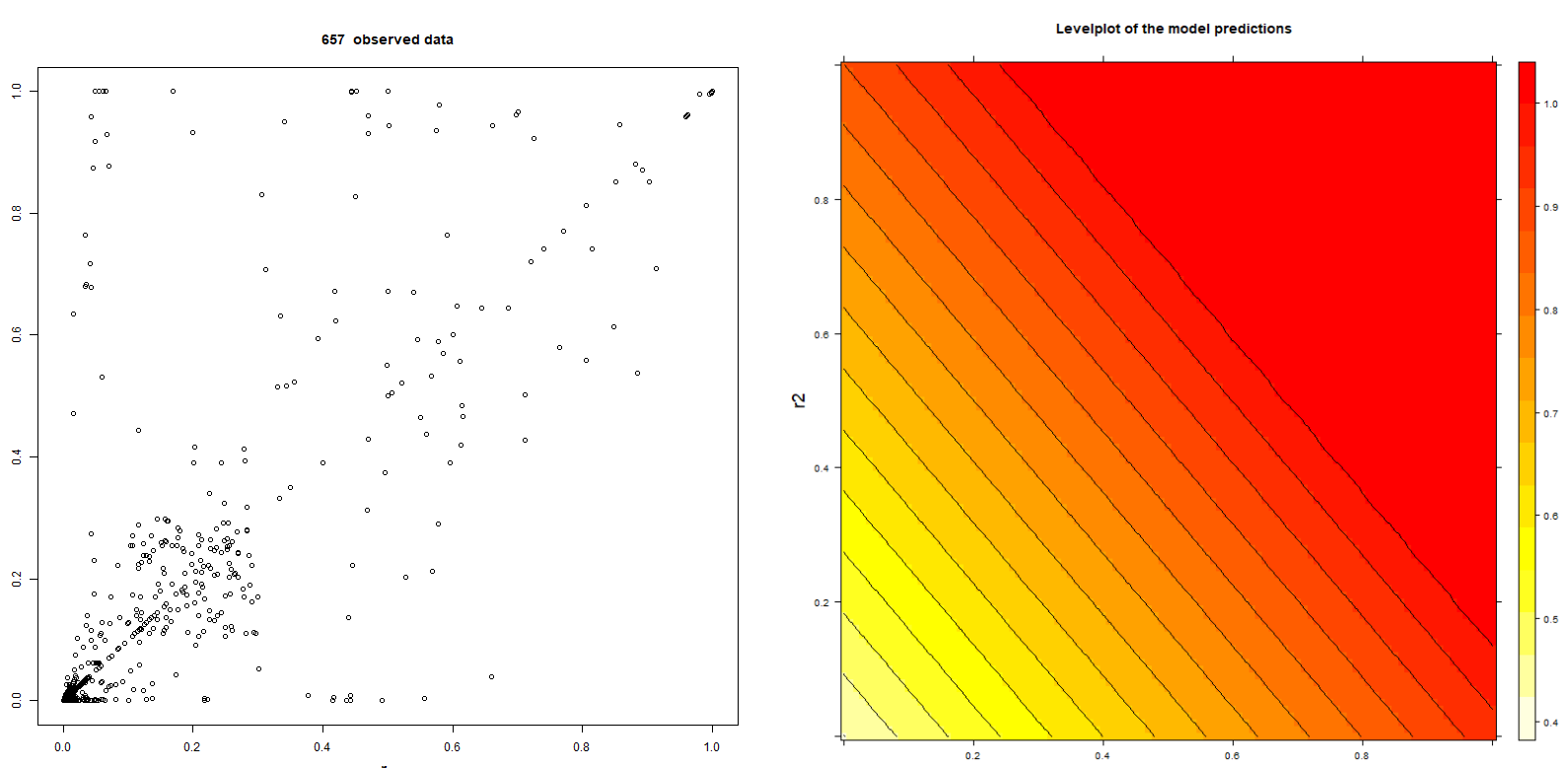
The following pictures are showing 657 data points of BehavioSecSession and BehavioSecTransaction plug-in risk scores (denoted by r₁ and r₂) from a nevisDetect test system and a level plot of the trained normalization:

Note that the data are not realistic, because the test system is frequently being used for demonstration purposes with a confidence threshold of 0.0.

The advantages of the ordinary least square normalization mode are:

• Training the model is fast, stable and also suited for a large training data set.
• The model parameters w and a can be interpreted by a human being.
• The Monotonicity property is fulfilled.

The disadvantages are:

• Using a linear regression function is an over-simplification.
• The Proximity property is in general not fulfilled.

Support vector regression normalization model

The normalization model described here is experimental.

A more advanced approach for solving the regression problem is the Support Vector Machine Regression (SV Regression). With this approach, also non-linear dependencies between the plug-in risk scores and the normalized risk score can be trained. The support vector regression normalization model (SVR-model) uses an approach with a radial kernel. The SV Regression has two hyperparameters:

• The box constraint parameter C.
• The hyperparameter γ in the radial kernel exp(-γ · ||r⁽ⁱ⁾ - r^(j)||²).

The hyperparameter γ is controlling the contribution of the support vectors to the predicted normalized risk score. In case of a large γ, the term exp(-γ · ||r⁽ⁱ⁾ - r||²) is only contributing if the support vector r⁽ⁱ⁾ is near to r. In case of a small γ, the term is also contributing if r⁽ⁱ⁾ is far away from r. Thus, it is possible to control the conflicting Monotonicity and Proximity properties by choosing appropriate values of γ and C. A large value of γ favors the Proximity property. The pictures below show the level plots of two trained normalization models, the first with γ = 0.1 and the second with γ = 0.01. For both models C = 10 and the 657 data points shown above have been used for training.

It would be desired to have a single hyperparameter in the range [0,1] with the hyperparameters γ and C being computed by the system. In the current version that is not possible; the hyperparameters γ and C were chosen by hand.